텐서플로우 모델 학습을 직접 구현하기
모델 컴파일
텐서플로우 모델은 model.compile()과 model.fit()으로 간단하게 모델 컴파일, 모델 피팅을 수행할 수 있습니다.
이 과정에서 텐서플로우 모델은 훈련용 데이터에 최적화 함수와 손실 함수를 취하여 파라미터를 업데이트합니다.
이 작업을 텐서플로우의 GradientTape을 이용하여 사용자 정의하겠습니다.
GradientTape은 연관된 연산을 기록하고, 자동 미분하여 기울기를 구해주는 API입니다.
GradientTape
GradienTape는 다음과 같이 사용합니다.
import tensorflow as tf

with tf.GradientTape() as tape:
  predictions = model(x)
  loss = loss_function(y, predictions)

gradients = tape.gradient(loss, model.trainable_variables)
with tf.GradientTape() as tape
Context 안에서 실행된 모든 연산을 tape에 기록하고,
tape.gradient(loss, x)
자동 미분한 기울기를 구합니다.
요구사항
모델 컴파일 및 모델 피팅을 대체하기 위하여 필요한 작업은 다음과 같습니다.
- Forward Propagation 수행
- Loss 계산
- Back Propagation 수행
- 1~3을 반복
Forward Propagation은 input layer부터 output layer까지 순서대로 연산하여 예측값을 구하는 작업이고,
Backward Propagation은 output layer부터 input layer까지 되돌아가며 가중치를 최적화하는 작업입니다.
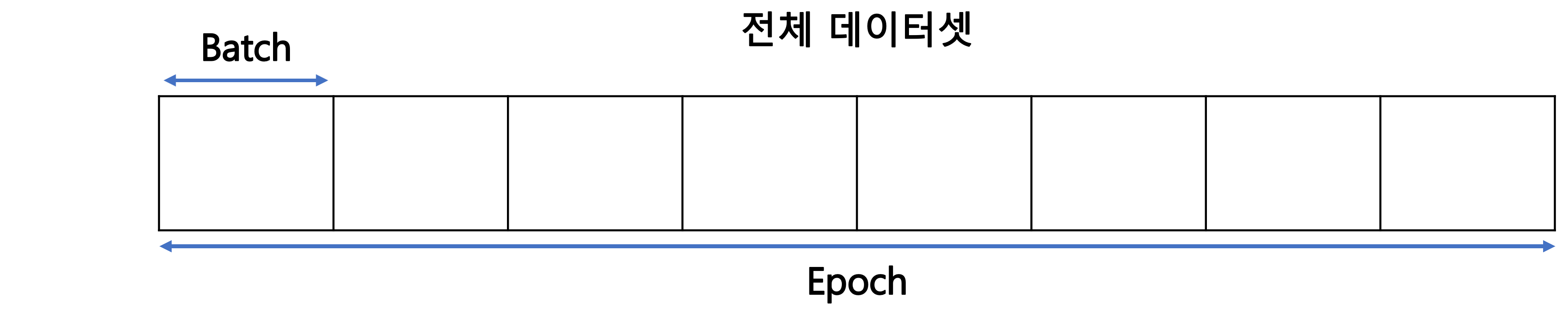
위 작업을 미니 배치 방식으로 epoch 수만큼 반복해야합니다.
코드
최적화 함수(adam)와 손실함수(cross entropy)를 정의합니다.
import tensorflow as tf

optimizer = tf.keras.optimizers.Adam()
loss_function = tf.keras.losses.SparseCategoricalCrossentropy()
학습 단계마다 Backward Propagation을 수행하는 함수를 작성합니다.
def train_step(features, labels):
    with tf.GradientTape() as tape:
        predictions = model(features)
        loss = loss_function(labels, predictions)

    gradients = tape.gradient(loss, model.trainable_variables)
    optimizer.apply_gradients(zip(gradients, model.trainable_variables))
    return loss
미니 배치 방식으로 작업을 반복하는 함수를 정의합니다.
def train_model(epochs = 5, batch_size = 32):
  for epoch in range(epochs):
    x_batch = []
    y_batch = []
    for step, (x, y) in enumerate(zip(x_train, y_train)):
      x_batch.append(x)
      y_batch.append(y)
      if (step % batch_size) == (batch_size - 1):
        loss = train_step(np.array(x_batch, dtype = np.float32),
                          np.array(y_batch, dtype = np.float32))
        x_batch = []
        y_batch = []

    print('Epoch %d: batch loss = %.4f' % (epoch, float(loss)))
실습
데이터를 준비하고, 모델을 생성합니다.
import tensorflow as tf
import numpy as np

# data
mnist = tf.keras.datasets.mnist
(x_train, y_train), (x_test, y_test) = mnist.load_data()
x_train, x_test = x_train / 255, x_test / 255 # rescaling

x_train = x_train[..., np.newaxis]
x_test = x_test[..., np.newaxis]

# build a model
model = tf.keras.Sequential([
    tf.keras.layers.Conv2D(32, 3, activation='relu'),
    tf.keras.layers.Conv2D(64, 3, activation='relu'),
    tf.keras.layers.Flatten(),
    tf.keras.layers.Dense(128, activation='relu'),
    tf.keras.layers.Dense(10, activation='softmax')
])
위에서 생성한 함수를 실행합니다.
train_model()
Epoch 0: batch loss = 0.0162
Epoch 1: batch loss = 0.0008
Epoch 2: batch loss = 0.0007
Epoch 3: batch loss = 0.0004
Epoch 4: batch loss = 0.0000
시험용 데이터로 정확도를 구합니다.
prediction = model.predict(x_test, batch_size=x_test.shape[0])
correct = sum(np.squeeze(y_test) == np.argmax(prediction, axis=1))
correct / len(y_test)
0.9872